Matrix Calculus for DeepLearning (Part3)
May 30, 2020

We have looked into Jacobian matrix, element wise operation, derivatives involving single expressions and vector sum reduction and chain rule in previous blog. Please through that, Blog 1, Blog 2.
The gradient of neuron activation
Let us compute the derivative of a typical neuron activation for a single neural network computation unit with respect to the model parameters, w and b
activation(x) = max(0, w . x + b)
This represents neuron with fully connected weights and relu.\ Let us compute derivative of ( w . x + b ) wrt w and b\ dot product w . x is summation of element wise multiplication of elements.\ Partial derivative of sum(w ⊗ x) can be calculated using chain rule using intermediate vector variable
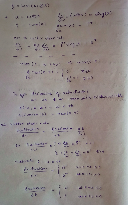
The above image use of the max(0, z) function call on scalar z just says to treat all negative z values as 0. The derivative of the max function is a piecewise function. When z ≤ 0, the derivative is 0 because z is a constant. When z > 0, the derivative of the max function is just the derivative of z, which is 1.
When the activation function clips affine function output z to 0, the derivative is zero with respect to any weight w i . When z > 0, it’s as if the max function disappears and we get just the derivative of z with respect to the weights.
The gradient of the neural network loss function
Training a neuron requires that we take the derivative of our loss or “cost” function with respect to the parameters of our model, w and b
We need to calculate gradient wrt weights and bias
Let X = [x 1 , x 2 , … , xN ] T (T means transpose)
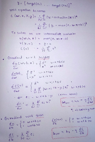
If the error is 0, then the gradient is zero and we have arrived at the minimum loss. If ei is some small positive difference, the gradient is a small step in the direction of x . If e 1 is large, the gradient is a large step in that direction. we want to reduce, not increase, the loss, which is why the gradient descent recurrence relation takes the negative of the gradient to update the current position.
Look at things like the shape of a vector (long or tall), is the variable scalar or vector, the dimensions of a matrix. Vectors are represented by bold letters\ After reading this blog please read paper, to get more understanding.\ Paper has unique way of explaining concepts, that is from simple to complex. when we reach the end of paper, we would solve ourself, because difficult expressions can be solved, since we have deep understanding of simple expressions.
First, we start with functions of simple parameters represented by f(x). Second,we move to functions of the form f(x,y,z). To calculate the derivatives of such functions, we use partial derivatives which are calculated with respect to specific parameters. Thirdly we move to scalar function of a vector of input parameters as f(x), wherein the partial derivatives of f(x) are represented as vectors. Lastly, we see f(x) to represent a set of scalar functions of the form f(x).
This is last part of blog, part3.
Thank you.
# Blog 11
